Pseudo Bulk Differential Expression Analysis
2023-11-09
Source:vignettes/2_pb_dgea.Rmd
2_pb_dgea.RmdPreliminaries
Data Availability
Raw sequencing data for this analysis is stored in GEO under accession number GSE211088.
The code used in this analysis has been deposited into Github, and can be available here.
Bioconductor packages
The differential expression (DE) analysis was carried out with edgeR. Remove Unwanted Variation (RUV) normalization is implemented in the RUVSeq package. To normalize raw data before RUV and to visualize the Principal Component Analysis (PCA) of UQ + RUV normalization, we used the EDASeq package. Some plots were visualized using the ggplot2 package. The Upset plot was visualized using the UpSetR and the ComplexUpset packages.
Differential expression analysis
For each neuronal cell-type with more than 500 cells, the differential gene expression analysis was carried out with a negative binomial generalized linear model (GLM) on pseudo-bulk samples.
Load data
UQ + RUV
Then, we normalized the raw counts with the upper-quartile method, using the betweenLaneNormalization function of the EDASeq package with option which=“upper”. To account for latent confounders, we computed a factor of unwanted variation on the normalized data, using the RUVs function of the RUVSeq package with k=2 and using as negative control genes a list of genes previously characterized as non-differential in sleep deprivation in a large microarray meta-analysis. Specifically, 10% of negative control genes were randomly selected to be used for evaluation and the remaining control genes were used to fit RUV normalization.
# UQ + RUV normalization
neg_ctrl <- read.table("SD_Negative_Controls.txt")
# The 10% of meta-analysis negative control genes were randomly
# selected.
set.seed(23)
random_ng <- sample(neg_ctrl$x, round(length(neg_ctrl$x) * 0.1))
# The remaining control genes were used to fit RUV
# normalization.
neg_ctrl <- neg_ctrl[!(neg_ctrl$x %in% random_ng), ]
neg_ctrl <- intersect(rownames(pb), neg_ctrl)

# UQ normalization
ct_counts <- lapply(pb_ct, function(x) as.matrix(counts(x)))
uq <- lapply(ct_counts, function(u) betweenLaneNormalization(u, which = "upper"))

# RUV normalization
ruv2_expr_data <- ruv2_w <- list()
for (i in seq_along(unique(pb$azimuth_labels))) {
    # A matrix specifying the replicates constructed
    groups <- makeGroups(pb_ct[[i]]$condition)

    # The matrix of normalized counts was saved in a list object
    ruv2_expr_data[[i]] <- RUVs(uq[[i]], cIdx = neg_ctrl, scIdx = groups,
        k = 2)
    # The factors of unwanted variation were saved in a list
    # object
    ruv2_w[[i]] <- ruv2_expr_data[[i]]$W
}
Differentially expressed genes identification
We then used the Bioconductor edgeR package to perform differential expression after filtering the lowly expressed genes with the filterByExpr function (with default parameters). The factor of unwanted variation was added in the design matrix. The differential gene expression analysis was computed with the function glmLRT by specifying “SD-HC” (Sleep Deprived vs Home Cage Control) as contrast and offset term equal to zero, since normalization was already carried out by the RUV factor.
res_uq_ruv2 <- df_uq_ruv2 <- list()
for (i in seq_along(unique(pb$azimuth_labels))) {
    y <- DGEList(counts(pb_ct[[i]]), samples = colData(pb_ct[[i]]))

    # The genes were filtered for each cell-type
    keep <- filterByExpr(y, group = pb_ct[[i]]$condition)
    y <- y[keep, ]
    # Upper-quartile normalization
    y <- calcNormFactors(y, method = "upperquartile")

    # Design Matrix
    design <- model.matrix(~0 + y$samples$condition + ruv2_w[[i]],
        y$samples)
    colnames(design) <- c("HC", "SD", "W_1", "W_2")

    y <- estimateDisp(y, design)

    fit <- glmFit(y, design)

    # Contrast creation (SD vs HC)
    contrast <- makeContrasts(SD - HC, levels = design)

    res_uq_ruv2[[i]] <- glmLRT(fit, contrast = contrast)

    df_uq_ruv2[[i]] <- as.data.frame(res_uq_ruv2[[i]]$table)
    df_uq_ruv2[[i]] <- df_uq_ruv2[[i]][order(df_uq_ruv2[[i]]$PValue),
        ]

    FDR <- as.data.frame(topTags(res_uq_ruv2[[i]], n = length(rownames(pb)))[,
        5])

    df_uq_ruv2[[i]] <- cbind(df_uq_ruv2[[i]], FDR)
    df_uq_ruv2[[i]] <- df_uq_ruv2[[i]][order(df_uq_ruv2[[i]]$FDR),
        ]
}
names(df_uq_ruv2) <- unique(pb$azimuth_labels)
Results
We used the Benjamini-Hochberg procedure to control for the false discovery rate (FDR), i.e., we considered as differentially expressed those genes that had an adjusted p-value less than 5%.
# N. of nuclei
n_nuclei <- matrix(pb$ncells, 11, 6, byrow = TRUE)
n_nuclei <- rowSums(n_nuclei)

# DEA results for differentially expressed genes were selected
df_degs <- lapply(df_uq_ruv2, function(u) u[u$FDR < 0.05, ])

# N. of DEGs
n_degs <- lapply(df_degs, function(u) length(rownames(u)))

posctrl <- read.table("Additional_File2_Positive_Controls.txt", header = TRUE)
# N. of DE positive control genes
n_de_posctrl <- lapply(df_degs, function(u) length(intersect(rownames(u),
    posctrl$Gene_ID)))
Scatter plot
We visualized the scatter plot of the logarithm of the number of nuclei and the logarithm of the number of differential genes expressed.
label_color <- c("Astro", "Car3", "Endo", "L2/3 IT CTX", "L4/5 IT CTX",
    "L5 IT CTX", "L5 PT CTX", "L5/6 NP CTX", "L6 CT CTX", "L6 IT CTX",
    "L6b CTX", "Lamp5", "Micro-PVM", "Oligo", "Pvalb", "SMC-Peri",
    "Sncg", "Sst", "Sst Chodl", "Vip", "VLMC")

subclass_color <- c("#957b46", "#5100FF", "#c95f3f", "#0BE652", "#00E5E5",
    "#50B2AD", "#0D5B78", "#3E9E64", "#2D8CB8", "#A19922", "#7044AA",
    "#DA808C", "#94AF97", "#744700", "#D93137", "#4c1130", "#ffff00",
    "#FF9900", "#B1B10C", "#B864CC", "#a9bd4f")

names(subclass_color) <- label_color

subclass_color <- data.frame(subclass_color)
subclass_color$Label <- rownames(subclass_color)
colnames(subclass_color) <- c("color", "Label")
rm_labels <- subclass_color[rownames(subclass_color) %in% intersect(rownames(subclass_color),
    levels(factor(pb$azimuth_labels))), ]

neuronal_color <- rm_labels$color
names(neuronal_color) <- rm_labels$Label

tab <- as.data.frame(cbind(n_nuclei, as.matrix(n_degs)))
colnames(tab) <- c("nuclei", "DEG")
tab$Label <- levels(factor(pb$azimuth_labels))
tab$DEG <- as.numeric(tab$DEG)
tab$nuclei <- as.numeric(tab$nuclei)

# Scatter plot of log(nuclei) vs log(DEGs)
ggplot(tab, aes(x = log(nuclei), y = log(DEG))) + geom_point(aes(color = Label),
    size = 3) + scale_color_manual(values = neuronal_color) + theme_classic() +
    theme(legend.position = "none", axis.text = element_text(size = 7),
        axis.title = element_text(size = 7)) + stat_smooth(method = "lm",
    formula = y ~ poly(x, 2), se = FALSE, col = "grey") + geom_label_repel(aes(label = Label),
    size = 2, box.padding = 0.5, point.padding = 0, segment.color = "grey50",
    min.segment.length = unit(1.5, "lines"), colour = neuronal_color)
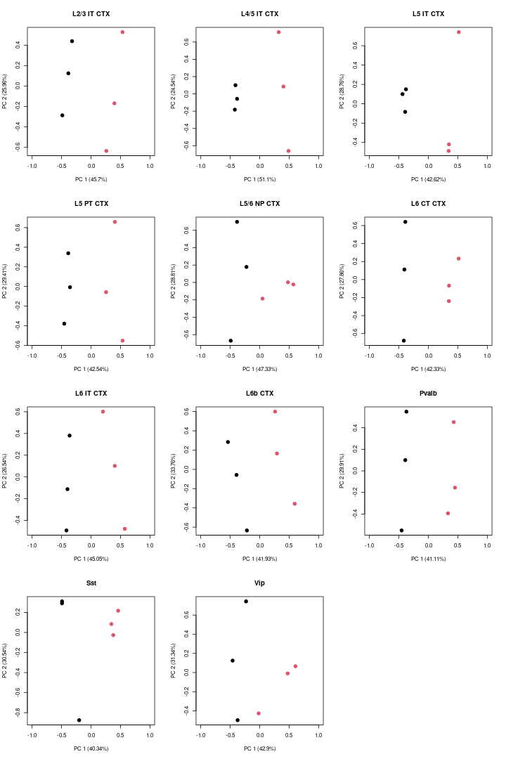
PCA
Then, we visualized the PCA for each cell-type.
label <- levels(factor(pb$azimuth_labels))
set_ct <- lapply(pb_ct, function(u) newSeqExpressionSet(as.matrix(round(counts(u))),
    phenoData = data.frame(colData(u), row.names = colnames(u))))
set_ct <- lapply(set_ct, function(u) betweenLaneNormalization(u, which = "upper"))

set_ruv2 <- list()
for (i in seq_along(unique(pb$azimuth_labels))) {
    # A matrix specifying the replicates constructed
    groups <- makeGroups(pb_ct[[i]]$condition)

    # k = 2 The matrix of normalized counts was saved in a list
    # object
    set_ruv2[[i]] <- RUVs(set_ct[[i]], cIdx = neg_ctrl, scIdx = groups,
        k = 2)

}
par(mfrow = c(4, 3))
for (i in seq_along(label)) {
    plotPCA(set_ruv2[[i]], xlim = c(-1, 1), label = FALSE, pch = 20,
        theme_size = 7, col = as.numeric(as.factor(set_ruv2[[i]]$condition)),
        cex = 2, main = paste(label[i], sep = " "))
}
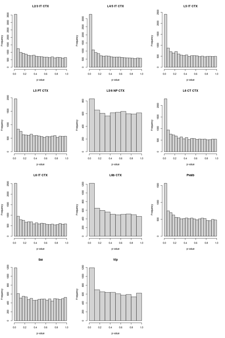
Volcano plot
We visualized the volcano plot and histogram for each cell-type.
## Volcano plot of all cell-types
for (i in seq_along(df_uq_ruv2)) {
    df_uq_ruv2[[i]]$Significance <- "No Significant"
    df_uq_ruv2[[i]]$Significance[df_uq_ruv2[[i]]$FDR < 0.05] <- "Significant"
    inter <- intersect(rownames(df_uq_ruv2[[i]][df_uq_ruv2[[i]]$FDR <
        0.05, ]), posctrl$Gene_ID)
    df_uq_ruv2[[i]]$Significance[rownames(df_uq_ruv2[[i]]) %in% inter] <- "SignificantPos"
}

p1 <- ggplot(data = df_uq_ruv2[[1]], aes(x = logFC, y = -log10(PValue),
    col = Significance)) + geom_point(data = df_uq_ruv2[[1]][(df_uq_ruv2[[1]]$Significance ==
    "Significant" | df_uq_ruv2[[1]]$Significance == "No Significant"),
    ], size = 1) + geom_point(data = df_uq_ruv2[[1]][df_uq_ruv2[[1]]$Significance ==
    "SignificantPos", ], size = 1) + xlim(-5, 5) + theme_classic(base_size = 7) +
    theme(legend.position = "none") + scale_color_manual(values = c(Significant = "black",
    `No Significant` = "grey", SignificantPos = "red")) + ggtitle("L2/3 IT CTX") +
    annotate("text", x = -4, y = 2.5, label = n_degs[[1]]) + annotate("text",
    x = -4, y = 0.5, label = n_de_posctrl[[1]], color = "red")

p2 <- ggplot(data = df_uq_ruv2[[2]], aes(x = logFC, y = -log10(PValue),
    col = Significance)) + geom_point(data = df_uq_ruv2[[2]][(df_uq_ruv2[[2]]$Significance ==
    "Significant" | df_uq_ruv2[[2]]$Significance == "No Significant"),
    ], size = 1) + geom_point(data = df_uq_ruv2[[2]][df_uq_ruv2[[2]]$Significance ==
    "SignificantPos", ], size = 1) + xlim(-5, 5) + theme_classic(base_size = 7) +
    theme(legend.position = "none") + scale_color_manual(values = c(Significant = "black",
    `No Significant` = "grey", SignificantPos = "red")) + ggtitle("L4/5 IT CTX") +
    annotate("text", x = -4, y = 2.5, label = n_degs[[2]]) + annotate("text",
    x = -4, y = 0.5, label = n_de_posctrl[[2]], color = "red")

p3 <- ggplot(data = df_uq_ruv2[[3]], aes(x = logFC, y = -log10(PValue),
    col = Significance)) + geom_point(data = df_uq_ruv2[[3]][(df_uq_ruv2[[3]]$Significance ==
    "Significant" | df_uq_ruv2[[3]]$Significance == "No Significant"),
    ], size = 1) + geom_point(data = df_uq_ruv2[[3]][df_uq_ruv2[[3]]$Significance ==
    "SignificantPos", ], size = 1) + xlim(-5, 5) + theme_classic(base_size = 7) +
    theme(legend.position = "none") + scale_color_manual(values = c(Significant = "black",
    `No Significant` = "grey", SignificantPos = "red")) + ggtitle("L5 IT CTX") +
    annotate("text", x = -4, y = 2, label = n_degs[[3]]) + annotate("text",
    x = -4, y = 0.5, label = n_de_posctrl[[3]], color = "red")

p4 <- ggplot(data = df_uq_ruv2[[4]], aes(x = logFC, y = -log10(PValue),
    col = Significance)) + geom_point(data = df_uq_ruv2[[4]][(df_uq_ruv2[[4]]$Significance ==
    "Significant" | df_uq_ruv2[[4]]$Significance == "No Significant"),
    ], size = 1) + geom_point(data = df_uq_ruv2[[4]][df_uq_ruv2[[4]]$Significance ==
    "SignificantPos", ], size = 1) + xlim(-5, 5) + theme_classic(base_size = 7) +
    theme(legend.position = "none") + scale_color_manual(values = c(Significant = "black",
    `No Significant` = "grey", SignificantPos = "red")) + ggtitle("L5 PT CTX") +
    annotate("text", x = -4, y = 2, label = n_degs[[4]]) + annotate("text",
    x = -4, y = 0.5, label = n_de_posctrl[[4]], color = "red")

p5 <- ggplot(data = df_uq_ruv2[[5]], aes(x = logFC, y = -log10(PValue),
    col = Significance)) + geom_point(data = df_uq_ruv2[[5]][(df_uq_ruv2[[5]]$Significance ==
    "Significant" | df_uq_ruv2[[5]]$Significance == "No Significant"),
    ], size = 1) + geom_point(data = df_uq_ruv2[[5]][df_uq_ruv2[[5]]$Significance ==
    "SignificantPos", ], size = 1) + xlim(-5, 5) + theme_classic(base_size = 7) +
    theme(legend.position = "none") + scale_color_manual(values = c(Significant = "black",
    `No Significant` = "grey", SignificantPos = "red")) + ggtitle("L5/6 NP CTX") +
    annotate("text", x = -4, y = 1.5, label = n_degs[[5]]) + annotate("text",
    x = -4, y = 0.5, label = n_de_posctrl[[5]], color = "red")

p6 <- ggplot(data = df_uq_ruv2[[6]], aes(x = logFC, y = -log10(PValue),
    col = Significance)) + geom_point(data = df_uq_ruv2[[6]][(df_uq_ruv2[[6]]$Significance ==
    "Significant" | df_uq_ruv2[[6]]$Significance == "No Significant"),
    ], size = 1) + geom_point(data = df_uq_ruv2[[6]][df_uq_ruv2[[6]]$Significance ==
    "SignificantPos", ], size = 1) + xlim(-5, 5) + theme_classic(base_size = 7) +
    theme(legend.position = "none") + scale_color_manual(values = c(Significant = "black",
    `No Significant` = "grey", SignificantPos = "red")) + ggtitle("L6 CT CTX") +
    annotate("text", x = -4, y = 2, label = n_degs[[6]]) + annotate("text",
    x = -4, y = 0.5, label = n_de_posctrl[[6]], color = "red")

p7 <- ggplot(data = df_uq_ruv2[[7]], aes(x = logFC, y = -log10(PValue),
    col = Significance)) + geom_point(data = df_uq_ruv2[[7]][(df_uq_ruv2[[7]]$Significance ==
    "Significant" | df_uq_ruv2[[7]]$Significance == "No Significant"),
    ], size = 1) + geom_point(data = df_uq_ruv2[[7]][df_uq_ruv2[[7]]$Significance ==
    "SignificantPos", ], size = 1) + xlim(-5, 5) + theme_classic(base_size = 7) +
    theme(legend.position = "none") + scale_color_manual(values = c(Significant = "black",
    `No Significant` = "grey", SignificantPos = "red")) + ggtitle("L6 IT CTX") +
    annotate("text", x = -4, y = 2, label = n_degs[[7]]) + annotate("text",
    x = -4, y = 0.5, label = n_de_posctrl[[7]], color = "red")

p8 <- ggplot(data = df_uq_ruv2[[8]], aes(x = logFC, y = -log10(PValue),
    col = Significance)) + geom_point(data = df_uq_ruv2[[8]][(df_uq_ruv2[[8]]$Significance ==
    "Significant" | df_uq_ruv2[[8]]$Significance == "No Significant"),
    ], size = 1) + geom_point(data = df_uq_ruv2[[8]][df_uq_ruv2[[8]]$Significance ==
    "SignificantPos", ], size = 1) + xlim(-5, 5) + theme_classic(base_size = 7) +
    theme(legend.position = "none") + scale_color_manual(values = c(Significant = "black",
    `No Significant` = "grey", SignificantPos = "red")) + ggtitle("L6b CTX") +
    annotate("text", x = -4, y = 1.5, label = n_degs[[8]]) + annotate("text",
    x = -4, y = 0.5, label = n_de_posctrl[[8]], color = "red")

p9 <- ggplot(data = df_uq_ruv2[[9]], aes(x = logFC, y = -log10(PValue),
    col = Significance)) + geom_point(data = df_uq_ruv2[[9]][(df_uq_ruv2[[9]]$Significance ==
    "Significant" | df_uq_ruv2[[9]]$Significance == "No Significant"),
    ], size = 1) + geom_point(data = df_uq_ruv2[[9]][df_uq_ruv2[[9]]$Significance ==
    "SignificantPos", ], size = 1) + xlim(-5, 5) + theme_classic(base_size = 7) +
    theme(legend.position = "none") + scale_color_manual(values = c(Significant = "black",
    `No Significant` = "grey", SignificantPos = "red")) + ggtitle("Pvalb") +
    annotate("text", x = -4, y = 1.5, label = n_degs[[9]]) + annotate("text",
    x = -4, y = 0.5, label = n_de_posctrl[[9]], color = "red")

p10 <- ggplot(data = df_uq_ruv2[[10]], aes(x = logFC, y = -log10(PValue),
    col = Significance)) + geom_point(data = df_uq_ruv2[[10]][(df_uq_ruv2[[10]]$Significance ==
    "Significant" | df_uq_ruv2[[10]]$Significance == "No Significant"),
    ], size = 1) + geom_point(data = df_uq_ruv2[[10]][df_uq_ruv2[[10]]$Significance ==
    "SignificantPos", ], size = 1) + xlim(-5, 5) + theme_classic(base_size = 7) +
    theme(legend.position = "none") + scale_color_manual(values = c(Significant = "black",
    `No Significant` = "grey", SignificantPos = "red")) + ggtitle("Sst") +
    annotate("text", x = -4, y = 1.5, label = n_degs[[10]]) + annotate("text",
    x = -4, y = 0.5, label = n_de_posctrl[[10]], color = "red")

p11 <- ggplot(data = df_uq_ruv2[[11]], aes(x = logFC, y = -log10(PValue),
    col = Significance)) + geom_point(data = df_uq_ruv2[[11]][(df_uq_ruv2[[11]]$Significance ==
    "Significant" | df_uq_ruv2[[11]]$Significance == "No Significant"),
    ], size = 1) + geom_point(data = df_uq_ruv2[[11]][df_uq_ruv2[[11]]$Significance ==
    "SignificantPos", ], size = 1) + xlim(-5, 5) + theme_classic(base_size = 7) +
    theme(legend.position = "none") + scale_color_manual(values = c(Significant = "black",
    `No Significant` = "grey", SignificantPos = "red")) + ggtitle("Vip") +
    annotate("text", x = -4, y = 1.5, label = n_degs[[11]]) + annotate("text",
    x = -4, y = 0.5, label = n_de_posctrl[[11]], color = "red")

# Blank space
p12 <- ggplot(data = df_uq_ruv2[[11]], aes(x = logFC, y = -log10(PValue),
    col = Significance)) + xlim(-5, 5) + theme_classic(base_size = 7) +
    theme(legend.position = "none")

(p1 | p2 | p3)/(p4 | p5 | p6)/(p7 | p8 | p9)/(p10 | p11 | plot_spacer())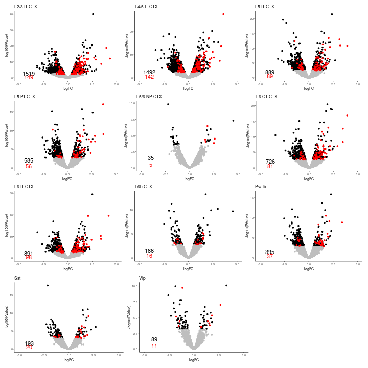
Upset plot
For Glutamatergic and GABAergic neurons, we used the upset function of the UpSetR package to identify the list of unique differentially expression genes for each cell-type.
df_degs <- lapply(df_uq_ruv2, function(u) rownames(u[u$FDR < 0.05, ]))

# Since the p-value distribution wasn't good, the L6b CTX label was removed
ll <- list("L2/3 IT CTX" = df_degs[[1]], "L4/5 IT CTX" = df_degs[[2]],
           "L5 IT CTX" = df_degs[[3]], "L5 PT CTX" = df_degs[[4]],
           "L6 CT CTX" = df_degs[[6]], "L6 IT CTX" = df_degs[[7]],
           "L6b CTX" = df_degs[[8]],
           "Pvalb" = df_degs[[9]], "Sst" = df_degs[[10]], "Vip" = df_degs[[11]])

df.edgeRList <- fromList(ll)

upset(df.edgeRList, colnames(df.edgeRList)[1:10],
      sort_intersections_by = c("degree", "cardinality"),
      sort_intersections = "ascending",
      name = "", width_ratio = 0.1, keep_empty_groups = TRUE,
      queries = list(
        upset_query(set = "L2/3 IT CTX", fill = "#0BE652"),
        upset_query(set = "L4/5 IT CTX", fill = "#00E5E5"),
        upset_query(set = "L5 IT CTX", fill = "#50B2AD"),
        upset_query(set = "L5 PT CTX", fill = "#0D5B78"),
        upset_query(set = "L6 CT CTX", fill = "#2D8CB8"),
        upset_query(set = "L6 IT CTX", fill = "#A19922"),
        upset_query(set = "L6b CTX", fill = "#7044AA"),
        upset_query(set = "Pvalb", fill = "#D93137"),
        upset_query(set = "Sst", fill = "#FF9900"),
        upset_query(set = "Vip", fill = "#B864CC")
      ),
      intersections = list(
        # Unique DEGs were visualized for each cell-type
        "L2/3 IT CTX", "L4/5 IT CTX", "L5 IT CTX", "L5 PT CTX",
        "L6 CT CTX", "L6 IT CTX", "L6b CTX", "Pvalb", "Sst", "Vip"
      ),
      base_annotations = list(
        "Intersection size" = (
          intersection_size(
            bar_number_threshold = 1, # show all numbers on top of bars
            width = 0.4,  # reduce width of the bars
            text = list(size = 2)
          )
          # add some space on the top of the bars
          + scale_y_continuous(expand = expansion(mult = c(0, 0.05)))
          + theme(
            # hide grid lines
            panel.grid.major = element_blank(),
            panel.grid.minor = element_blank(),
            # show axis lines
            axis.line = element_line(colour = "black")
          )
        )
      ),
      stripes = upset_stripes(
        geom = geom_segment(size = 3),
        colors = c("grey95", "white")
      ),
      matrix = intersection_matrix(
        geom = geom_point(
          shape = "circle filled",
          size = 2,
          stroke = 0
        )
      ),
      set_sizes = (
        upset_set_size(geom = geom_bar(width = 0.5), filter_intersections = TRUE)
        + theme(
          axis.line.x = element_line(colour = "black"),
          axis.ticks.x = element_line()
        )
      ),
      themes = upset_default_themes(text = element_text(size = 7, color = "black"))) +
  theme(plot.background = element_blank(),
        panel.grid.major = element_blank(),
        panel.grid.minor = element_blank(),
        panel.border = element_blank())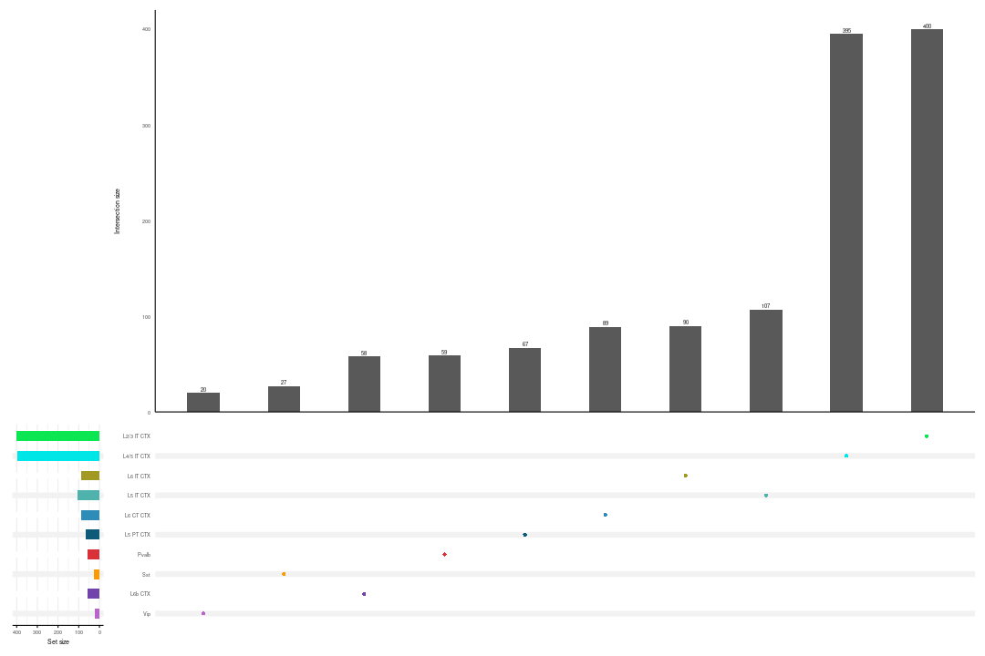
Session Info
## R version 4.2.0 (2022-04-22)
## Platform: x86_64-pc-linux-gnu (64-bit)
## Running under: Ubuntu 20.04.4 LTS
##
## Matrix products: default
## BLAS:   /usr/lib/x86_64-linux-gnu/blas/libblas.so.3.9.0
## LAPACK: /usr/lib/x86_64-linux-gnu/lapack/liblapack.so.3.9.0
##
## locale:
##  [1] LC_CTYPE=en_US.UTF-8       LC_NUMERIC=C
##  [3] LC_TIME=en_US.UTF-8        LC_COLLATE=en_US.UTF-8
##  [5] LC_MONETARY=en_US.UTF-8    LC_MESSAGES=en_US.UTF-8
##  [7] LC_PAPER=en_US.UTF-8       LC_NAME=C
##  [9] LC_ADDRESS=C               LC_TELEPHONE=C
## [11] LC_MEASUREMENT=en_US.UTF-8 LC_IDENTIFICATION=C
##
## attached base packages:
## [1] stats4    stats     graphics  grDevices utils     datasets
## [7] methods   base
##
## other attached packages:
##  [1] patchwork_1.1.2
##  [2] ComplexUpset_1.3.3
##  [3] UpSetR_1.4.0
##  [4] ggrepel_0.9.3
##  [5] RUVSeq_1.32.0
##  [6] EDASeq_2.32.0
##  [7] ShortRead_1.56.1
##  [8] GenomicAlignments_1.34.0
##  [9] Rsamtools_2.14.0
## [10] Biostrings_2.66.0
## [11] XVector_0.38.0
## [12] BiocParallel_1.32.5
## [13] GEOquery_2.66.0
## [14] BiocManager_1.30.19
## [15] knitr_1.42
## [16] BiocStyle_2.26.0
## [17] rmarkdown_2.20
## [18] dplyr_1.0.10
## [19] AllenInstituteBrainData_0.99.1
## [20] edgeR_3.40.2
## [21] limma_3.54.1
## [22] muscat_1.12.1
## [23] biomaRt_2.54.0
## [24] ggplot2_3.3.6
## [25] pbmcsca.SeuratData_3.0.0
## [26] mousecortexref.SeuratData_1.0.0
## [27] SeuratData_0.2.2
## [28] Azimuth_0.4.6
## [29] shinyBS_0.61.1
## [30] SeuratObject_4.1.3
## [31] Seurat_4.3.0
## [32] scDblFinder_1.12.0
## [33] scran_1.26.2
## [34] scuttle_1.8.4
## [35] EnsDb.Mmusculus.v79_2.99.0
## [36] ensembldb_2.22.0
## [37] AnnotationFilter_1.22.0
## [38] GenomicFeatures_1.50.4
## [39] AnnotationDbi_1.60.0
## [40] SingleCellExperiment_1.20.0
## [41] SummarizedExperiment_1.28.0
## [42] Biobase_2.58.0
## [43] GenomicRanges_1.50.2
## [44] GenomeInfoDb_1.34.9
## [45] IRanges_2.32.0
## [46] S4Vectors_0.36.1
## [47] BiocGenerics_0.44.0
## [48] MatrixGenerics_1.10.0
## [49] matrixStats_0.63.0
##
## loaded via a namespace (and not attached):
##   [1] rsvd_1.0.5                ica_1.0-3
##   [3] ps_1.7.2                  rprojroot_2.0.3
##   [5] foreach_1.5.2             lmtest_0.9-40
##   [7] crayon_1.5.2              rbibutils_2.2.13
##   [9] MASS_7.3-58.2             rhdf5filters_1.10.0
##  [11] nlme_3.1-162              backports_1.4.1
##  [13] rlang_1.0.6               ROCR_1.0-11
##  [15] irlba_2.3.5.1             callr_3.7.3
##  [17] nloptr_2.0.3              scater_1.26.1
##  [19] filelock_1.0.2            xgboost_1.7.3.1
##  [21] rjson_0.2.21              bit64_4.0.5
##  [23] glue_1.6.2                sctransform_0.3.5
##  [25] processx_3.8.0            pbkrtest_0.5.2
##  [27] parallel_4.2.0            vipor_0.4.5
##  [29] spatstat.sparse_3.0-0     SeuratDisk_0.0.0.9020
##  [31] shinydashboard_0.7.2      spatstat.geom_3.0-6
##  [33] tidyselect_1.2.0          usethis_2.1.6
##  [35] fitdistrplus_1.1-8        variancePartition_1.28.4
##  [37] XML_3.99-0.13             tidyr_1.2.1
##  [39] zoo_1.8-11                xtable_1.8-4
##  [41] magrittr_2.0.3            evaluate_0.20
##  [43] Rdpack_2.4                cli_3.6.0
##  [45] zlibbioc_1.44.0           hwriter_1.3.2.1
##  [47] miniUI_0.1.1.1            sp_1.6-0
##  [49] aod_1.3.2                 tinytex_0.44
##  [51] shiny_1.7.4               BiocSingular_1.14.0
##  [53] xfun_0.37                 clue_0.3-64
##  [55] pkgbuild_1.4.0            cluster_2.1.4
##  [57] caTools_1.18.2            KEGGREST_1.38.0
##  [59] clusterGeneration_1.3.7   tibble_3.1.8
##  [61] listenv_0.9.0             png_0.1-8
##  [63] future_1.31.0             withr_2.5.0
##  [65] bitops_1.0-7              plyr_1.8.8
##  [67] cellranger_1.1.0          dqrng_0.3.0
##  [69] pillar_1.8.1              gplots_3.1.3
##  [71] GlobalOptions_0.1.2       cachem_1.0.6
##  [73] fs_1.6.1                  hdf5r_1.3.8
##  [75] GetoptLong_1.0.5          RUnit_0.4.32
##  [77] DelayedMatrixStats_1.20.0 vctrs_0.4.1
##  [79] ellipsis_0.3.2            generics_0.1.3
##  [81] devtools_2.4.5            tools_4.2.0
##  [83] remaCor_0.0.11            beeswarm_0.4.0
##  [85] munsell_0.5.0             DelayedArray_0.24.0
##  [87] pkgload_1.3.2             fastmap_1.1.0
##  [89] compiler_4.2.0            abind_1.4-5
##  [91] httpuv_1.6.8              rtracklayer_1.58.0
##  [93] sessioninfo_1.2.2         plotly_4.10.1
##  [95] GenomeInfoDbData_1.2.9    gridExtra_2.3
##  [97] glmmTMB_1.1.5             lattice_0.20-45
##  [99] deldir_1.0-6              utf8_1.2.3
## [101] later_1.3.0               BiocFileCache_2.6.0
## [103] jsonlite_1.8.4            scales_1.2.1
## [105] ScaledMatrix_1.6.0        pbapply_1.7-0
## [107] sparseMatrixStats_1.10.0  lazyeval_0.2.2
## [109] promises_1.2.0.1          doParallel_1.0.17
## [111] R.utils_2.12.2            latticeExtra_0.6-30
## [113] goftest_1.2-3             spatstat.utils_3.0-1
## [115] reticulate_1.28           cowplot_1.1.1
## [117] blme_1.0-5                statmod_1.5.0
## [119] Rtsne_0.16                uwot_0.1.14
## [121] igraph_1.4.0              HDF5Array_1.26.0
## [123] survival_3.5-0            numDeriv_2016.8-1.1
## [125] yaml_2.3.7                htmltools_0.5.4
## [127] memoise_2.0.1             profvis_0.3.7
## [129] BiocIO_1.8.0              locfit_1.5-9.7
## [131] viridisLite_0.4.1         digest_0.6.31
## [133] assertthat_0.2.1          RhpcBLASctl_0.21-247.1
## [135] mime_0.12                 rappdirs_0.3.3
## [137] RSQLite_2.2.20            future.apply_1.10.0
## [139] remotes_2.4.2             data.table_1.14.6
## [141] urlchecker_1.0.1          blob_1.2.3
## [143] R.oo_1.25.0               labeling_0.4.2
## [145] splines_4.2.0             Rhdf5lib_1.20.0
## [147] googledrive_2.0.0         ProtGenerics_1.30.0
## [149] RCurl_1.98-1.10           broom_1.0.3
## [151] hms_1.1.2                 rhdf5_2.42.0
## [153] colorspace_2.1-0          ggbeeswarm_0.7.1
## [155] shape_1.4.6               Rcpp_1.0.10
## [157] RANN_2.6.1                mvtnorm_1.1-3
## [159] circlize_0.4.15           fansi_1.0.4
## [161] tzdb_0.3.0                parallelly_1.34.0
## [163] R6_2.5.1                  grid_4.2.0
## [165] ggridges_0.5.4            lifecycle_1.0.3
## [167] formatR_1.14              bluster_1.8.0
## [169] curl_5.0.0                googlesheets4_1.0.1
## [171] minqa_1.2.5               leiden_0.4.3
## [173] Matrix_1.5-3              desc_1.4.2
## [175] RcppAnnoy_0.0.20          RColorBrewer_1.1-3
## [177] iterators_1.0.14          spatstat.explore_3.0-6
## [179] TMB_1.9.2                 stringr_1.5.0
## [181] htmlwidgets_1.6.1         beachmat_2.14.0
## [183] polyclip_1.10-4           purrr_0.3.5
## [185] mgcv_1.8-41               ComplexHeatmap_2.14.0
## [187] globals_0.16.2            spatstat.random_3.1-3
## [189] progressr_0.13.0          codetools_0.2-19
## [191] metapod_1.6.0             gtools_3.9.4
## [193] prettyunits_1.1.1         dbplyr_2.3.0
## [195] R.methodsS3_1.8.2         gtable_0.3.1
## [197] DBI_1.1.3                 aroma.light_3.28.0
## [199] highr_0.10                tensor_1.5
## [201] httr_1.4.4                KernSmooth_2.23-20
## [203] stringi_1.7.12            presto_1.0.0
## [205] progress_1.2.2            farver_2.1.1
## [207] reshape2_1.4.4            annotate_1.76.0
## [209] viridis_0.6.2             DT_0.27
## [211] xml2_1.3.3                boot_1.3-28.1
## [213] shinyjs_2.1.0             BiocNeighbors_1.16.0
## [215] lme4_1.1-31               restfulr_0.0.15
## [217] interp_1.1-3              readr_2.1.4
## [219] geneplotter_1.76.0        scattermore_0.8
## [221] DESeq2_1.38.3             bit_4.0.5
## [223] jpeg_0.1-10               spatstat.data_3.0-0
## [225] pkgconfig_2.0.3           gargle_1.3.0
## [227] lmerTest_3.1-3